
Simply supported beam calculator
This tool calculates the static response of simply supported beams under various loading scenarios. The tool calculates and plots diagrams for these quantities:
- reactions
- bending moments
- transverse shear forces
- deflections
- slopes
Please take in mind that the assumptions of Euler-Bernoulli beam theory are adopted, the material is elastic and the cross section is constant over the entire beam span (prismatic beam).
Units: | |||||
| 1 | 2 | 3 | 4 |
Structure | |||
L = | |||
Optional properties, required only for deflection/slope results: | |||
E = | |||
I = | |||
| 1 | 2 | 3 | 4 | |||||||||||||||||||||||||||||||||||||||||||||||||||||||||||||||||||||||||||||||||||||||||||||||
Imposed loading: | ||||||||||||||||||||||||||||||||||||||||||||||||||||||||||||||||||||||||||||||||||||||||||||||||||

| 1 | 2 | 3 | 4 |
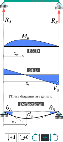
Results: | |||
Reactions: | |||
RA = | |||
RB = | |||
Bending Moment: | |||
Mu = | |||
xm = | |||
Transverse Shear Force: | |||
Vu = | |||
xv = | |||
Deflection: | |||
du = | |||
xd = | |||
Slopes: | |||
θA = | |||
θB = | |||
 |
| 1 | 2 | 3 | 4 |
Request results at a specific point: | |||
x = | |||
M(x) = | |||
V(x) = | |||
d(x) = | |||
θ(x) = | |||
| 1 | 2 | ||
Diagrams | |||
ADVERTISEMENT
Background
Table of contents
Introduction
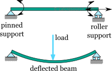
The simply supported beam is one of the most simple structures. It features only two supports, one at each end. One pinned support and a roller support. Both of them inhibit any vertical movement, allowing on the other hand, free rotations around them. The roller support also permits the beam to expand or contract axially, though free horizontal movement is prevented by the other support.
Removing any of the supports or inserting an internal hinge, would render the simply supported beam to a mechanism, that is body the moves without restriction in one or more directions. Obviously this is unwanted for a load carrying structure. Therefore, the simply supported beam offers no redundancy in terms of supports. If a local failure occurs the whole structure would collapse. These type of structures, that offer no redundancy, are called critical or determinant structures. To the contrary, a structure that features more supports than required to restrict its free movements is called redundant or indeterminate structure.
Assumptions
The static analysis of any load carrying structure involves the estimation of its internal forces and moments, as well as its deflections. Typically, for a plane structure, with in plane loading, the internal actions of interest are the axial force , the transverse shear force and the bending moment . For a simply supported beam that carries only transverse loads, the axial force is always zero, therefore it is often neglected. The calculated results in the page are based on the following assumptions:
- The material is homogeneous and isotropic (in other words its characteristics are the same in ever point and towards any direction)
- The material is linear elastic
- The loads are applied in a static manner (they do not change with time)
- The cross section is the same throughout the beam length
- The deflections are small
- Every cross-section that initially is plane and also normal to the longitudinal axis, remains plane and and normal to the deflected axis too. This is the case when the cross-section height is quite smaller than the beam length (10 times or more) and also the cross-section is not multi layered (not a sandwich type section).
The last two assumptions satisfy the kinematic requirements for the Euler Bernoulli beam theory that is adopted here too.
Sign convention
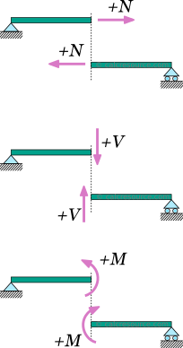
For the calculation of the internal forces and moments, at any section cut of the beam, a sign convention is necessary. The following are adopted here:
- The axial force is considered positive when it causes tension to the part
- The shear force is positive when it causes a clock-wise rotation of the part.
- The bending moment is positive when it causes tension to the lower fiber of the beam and compression to the top fiber.
These rules, though not mandatory, are rather universal. A different set of rules, if followed consistently would also produce the same physical results.
Symbols
- : the material modulus of elasticity (Young's modulus)
- : the moment of inertia of the cross-section around the elastic neutral axis of bending
- : the total beam span
- : support reaction
- : deflection
- : bending moment
- : transverse shear force
- : slope
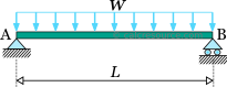
Simply supported beam with uniform distributed load
The load w is distributed throughout the beam span, having constant magnitude and direction. Its dimensions are force per length. The total amount of force applied to the beam is , where the span length. Either the total force or the distributed force per length may be given, depending on the circumstances.
In the following table, the formulas describing the static response of the simple beam under a uniform distributed load are presented.
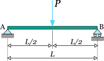
Simply supported beam with point force in the middle
The force is concentrated in a single point, located in the middle of the beam. In practice however, the force may be spread over a small area, although the dimensions of this area should be substantially smaller than the beam span length. In the close vicinity of the force application, stress concentrations are expected and as result the response predicted by the classical beam theory is maybe inaccurate. This is only a local phenomenon however. As we move away from the force location, the results become valid, by virtue of the Saint-Venant principle.
In the following table, the formulas describing the static response of the simple beam under a concentrated point force , imposed in the middle, are presented.
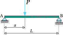
Simply supported beam with point force at a random position
The force is concentrated in a single point, anywhere across the beam span. In practice however, the force may be spread over a small area. In order to consider the force as concentrated, though, the dimensions of the application area should be substantially smaller than the beam span length. In the close vicinity of the force, stress concentrations are expected and as result the response predicted by the classical beam theory maybe inaccurate. This is only a local phenomenon however, and as we move away from the force location, the discrepancy of the results becomes negligible.
In the following table, the formulas describing the static response of the simple beam under a concentrated point force , imposed at a random distance from the left end, are presented.
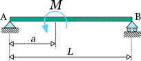
Simply supported beam with point moment
In this case, a moment is imposed in a single point of the beam, anywhere across the beam span. In practical terms, it could be a force couple, or a member in torsion, connected out of plane and perpendicular to the beam.
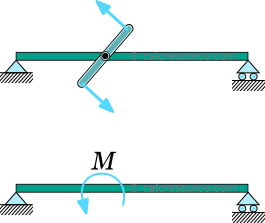
At any case, the moment application area should spread to a small length of the beam, so that it can be successfully idealized as a concentrated moment to a point. Although in the close vicinity the application area, the predicted results through the classical beam theory are expected to be inaccurate (due to stress concentrations and other localized effects), as we move away, the predicted results are perfectly valid, as stated by the Saint-Venant principle.
In the following table, the formulas describing the static response of the simple beam under a concentrated point moment , imposed at a distance from the left end, are presented.
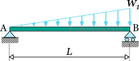
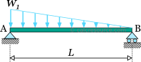
Simply supported beam with triangular load
The load is distributed throughout the beam span, however, its magnitude is not constant but is varying linearly, starting from zero at the left end to its peak value at the right end. The dimensions of are force per length. The total amount of force applied to the beam is , where the span length.
In the following table, the formulas describing the static response of the simple beam under a linearly varying (triangular) distributed load, ascending from the left to the right, are presented.
Simply supported beam with trapezoidal load
The load is distributed throughout the beam span, having linearly varying magnitude, starting from at the left end, to at the right end. The dimensions of and are force per length. The total amount of force applied to the beam is , where the span length.
In the following table, the formulas describing the static response of the simple beam under a varying distributed load, of trapezoidal form, are presented.
Simply supported beam with linearly varying distributed load (trapezoidal)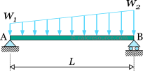 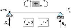 | |
|---|---|
| Quantity | Formula |
| Reactions: | |
| End slopes: | |
| Bending moment at x: | |
| Shear force at x: | |
| Deflection at x: | |
| Slope at x: | |
where: | |
Simply supported beam with slab-type trapezoidal load distribution
This load distribution is typical for the beams in the perimeter of a slab. The distribution is of trapezoidal shape, with maximum magnitude at the interior of the beam, while at its two ends it becomes zero. The dimensions of (\w\) are force per length. The total amount of force applied to the beam is , where the span length and , the lengths at the left and right side of the beam respectively, where the load distribution is varying (triangular).
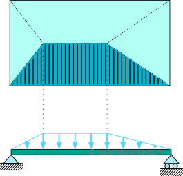
In the following table, the formulas describing the static response of the simple beam under a trapezoidal load distribution, as depicted in the schematic above, are presented.
Simply supported beam with trapezoidal load distribution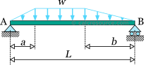 | |
|---|---|
| Quantity | Formula |
| Reactions: | |
| End slopes: | |
| Bending moment at x: | |
| Shear force at x: | |
| Deflection at x: | |
| Slope at x: | |
where: | |
Simply supported beam with partially distributed uniform load
The load is distributed to a part of the beam span, with constant magnitude , while the remaining span is unloaded. The dimensions of are force per length. The total amount of force applied to the beam is , where the span length and , the unloaded lengths at the left and right side of the beam, respectively.
In the following table, the formulas describing the static response of the simple beam, under a partially distributed uniform load, are presented.
Simply supported beam with partially distributed uniform load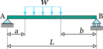 | |
|---|---|
| Quantity | Formula |
| Reactions: | |
| End slopes: | |
| Bending moment at x: | |
| Shear force at x: | |
| Deflection at x: | |
| Slope at x: | |
where: | |
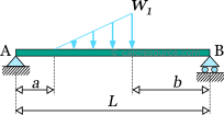
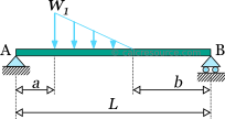
Simply supported beam with partially distributed trapezoidal load
The load is distributed to a part of the beam span, having linearly varying magnitude from to , while the remaining span is unloaded. The dimensions of and are force per length. The total amount of force applied to the beam is , where the span length and , the unloaded lengths at the left and right side of the beam respectively.
In the following table, the formulas describing the static response of the simple beam, under a partially distributed trapezoidal load, are presented.
Simply supported beam with partially distributed linearly varying load (trapezoidal)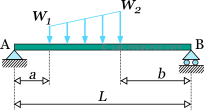 | |
|---|---|
| Quantity | Formula |
| Reactions: | |
| End slopes: | |
| Bending moment at x: | |
| Shear force at x: | |
| Deflection at x: | |
| Slope at x: | |
where: | |